This guide outlines the process of building a book recommendation system using distributed computing with Sklearn and Pandas, integrated into a fully deployed web application with Flask. It features K-Means clustering and Gaussian Mixture Modeling for content filtering to deliver personalized book recommendations.

Have you ever found yourself so mesmerized by a book that you wished there were more similar content out there? For many of us book lovers, this isn’t just a desire—it’s a necessity. Fortunately, with the advancements in machine learning and data science, we now have the privilege of receiving recommendations tailored to our interests. In the world of AI, this is known as a “Recommendation System.” These systems are widely used by e-commerce and entertainment companies such as Amazon and Netflix to increase user engagement, loyalty, satisfaction, and ultimately, the company’s profit.
One popular approach to recommendation systems is collaborative filtering, a technique that predicts items a user might like based on the reactions of similar users. Collaborative filtering is basically a user-based filtering.
In the user-based approach, we leverage the opinions of people who share similar interests with you. For example, if you and a friend both enjoy the book Atomic Habits by James Clear, and your friend also likes The Compound Effect by Darren Hardy, chances are you’ll like that book too! Companies rely on user feedback and ratings to suggest contents to others with similar tastes. Simply put, if Person A and Person B both like content C, and Person B likes content D, the system will recommend content D to Person A.
Another approach to recommendation system is called content-based filtering which focuses solely on the contents themselves, identifying which contents are most similar to what the user already enjoys.
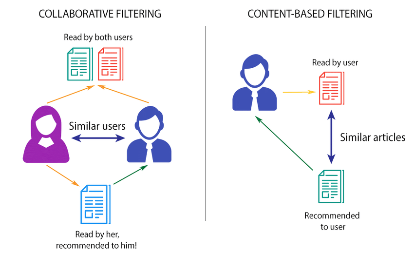
In this blog, we’ll implement content-based filtering. Given the name of a book chosen by our user, we’ll provide 10 suggested books that we think the user might also enjoy. How will we do this? By analyzing a pool of book titles, each ranked by multiple users, we’ll identify which books are similar to the one the user likes, then suggest those titles, assuming the user will enjoy them as well.
Importing Libraries
# Data manipulation
import numpy as np
import pandas as pd

# File handling
import os
import pickle

# Time management
import time

# Data visualization
import seaborn as sns
import matplotlib.pyplot as plt

# Machine learning
from sklearn.cluster import KMeans
from sklearn.decomposition import TruncatedSVD
from sklearn.model_selection import train_test_split
from sklearn.metrics.pairwise import cosine_similarity
from sklearn.metrics import silhouette_score
from sklearn.mixture import GaussianMixture
Loading Data
We’re using the Book Recommendation Dataset from Kaggle. Within this dataset, there are several files, but we only need books.csv and ratings.csv. Together, these files provide the ratings of over 1 million users on more than 270,000 books, with no duplicated rows in either dataset. Both files share a common column, ISBN, which we’ll use to merge them into one comprehensive dataset. This will make our analysis much smoother and more efficient.
if you are on Kaggle, use the following commands to load your data:
books_df = pd.read_csv('/kaggle/input/book-recommendation-dataset/Books.csv')
ratings_df = pd.read_csv('/kaggle/input/book-recommendation-dataset/Ratings.csv')
And if on Google Colab:
from google.colab import drive
drive.mount('/content/drive')

path = '/path/to/your/dataset/folder'

# List all CSV files in the directory
csv_files = [file for file in os.listdir(path) if file.endswith('.csv')]

# Create a dictionary to store the DataFrames
dataframes = {}

# Read each CSV file into a DataFrame and store it in the dictionary
for file in csv_files:
    # Extract the base name of the file (without extension) to use as the key
    base_name = os.path.splitext(file)[0]

    # Read the CSV file into a DataFrame
    dataframes[base_name] = pd.read_csv(os.path.join(path, file), header=True, inferSchema=True)
    # dataframes[base_name] = pd.read_csv(os.path.join(path, file))

# Display the first few rows of each DataFrame
for name, df in dataframes.items():
    print(f"DataFrame: {name}")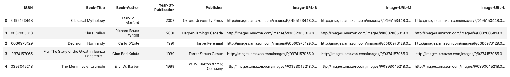
Data Preprocessing
The maximum rating a user can give to a book is 10, with 11 distinct rating options ranging from 0 to 10, where a higher rating indicates greater interest and zero means no rating.
As we merge the two datasets, books_df and ratings_df, we’ll notice that many items have no rating, resulting in null values. These null values indicate that the user did not rate that particular book. This situation makes our matrix sparse. Since we need to work exclusively with numerical data, we will replace these null values with zeros, signifying that the user did not rate the book.
# Calculate the maximum rating and find the unique ratings
print(ratings_df['Book-Rating'].max(), ratings_df['Book-Rating'].unique())

ratings_df.head(3)
print(f'Book dataframe\'s shape is {books_df.shape}')
print('Ratings\'s shape is: {}'.format(ratings_df.shape))![]()
print('Null values in books dataframe are as follows:')
print('**********************************************')
print(books_df.isnull().sum())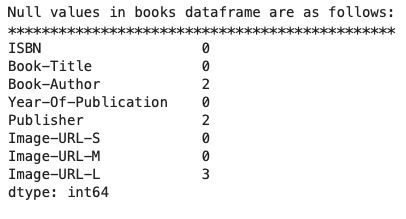
print('Null values in ratings dataframe are as follows:')
print('************************************************')
print(ratings_df.isnull().sum())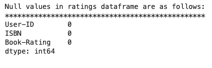
print('Number of duplicated values in books_df')
print('***************************************')

print(books_df.duplicated().sum())
print('Number of duplicated values in ratings_df')
print('*****************************************')

print(ratings_df.duplicated().sum())
As mentioned earlier, we merge the two datasets on the ISBN column. To ensure more reliable results, we will filter our data to include only users who have rated more than 100 books and books that have received more than 50 votes. Entries that don’t meet these criteria will be dropped from the dataset.
df = books_df.merge(ratings_df, on='ISBN')

user_prune = df.groupby('User-ID')['Book-Rating'].count() > 100
user_and_rating = user_prune[user_prune].index # outputs the User-IDs for users that rate more than 100 books

filtered_rating = df[df['User-ID'].isin(user_and_rating)]

rating_prune = df.groupby('Book-Title')['Book-Rating'].count() >= 50
famous_books = rating_prune[rating_prune].index

final_rating = filtered_rating[filtered_rating['Book-Title'].isin(famous_books)]
Pivot Table
Here, we are creating an item-based filtering system, which means constructing a table where Book-Title serve as row and User-ID as column.
book_pivot_table = final_rating.pivot_table(index='Book-Title', columns='User-ID', values='Book-Rating')

book_pivot_table.fillna(0, inplace=True)

print('datset dimension: ', (book_pivot_table.shape))
book_pivot_table.head(5)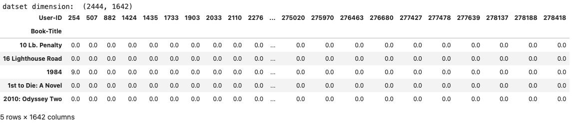
Notice how the number of users has shrunk from over a million to just 1,642. This highlights that only 0.14% of users rated more than 100 books, and only 0.9% of books were rated more than 50 times by these avid readers.
Dimensionality Reduction
Even with this significant reduction in dimensionality, our dataset still consumes a considerable amount of memory, making it computationally expensive to process. To address this, we can further reduce the matrix’s dimensions (specifically, the number of users) to decrease memory usage and speed up the training process. For this, we’ll use Truncated Singular Value Decomposition (SVD).
Truncated SVD is a matrix factorization technique similar to Principal Component Analysis (PCA). The key difference is that Truncated SVD operates directly on the data matrix, while PCA is applied to the covariance matrix. Truncated SVD factorizes the data matrix, truncating it to a specified number of columns, which effectively reduces the complexity of the data.
Read more at: TruncatedSVD
tsvd = TruncatedSVD(n_components=200, random_state=42) # reduce the dimentionality - similar to PCA
book_pivot_table_tsvd = tsvd.fit_transform(book_pivot_table)print('Original number of features before dimensionality reduction: ', (book_pivot_table.count(), len(book_pivot_table.columns)))
print('Number of features after dimensionality reduction: ', book_pivot_table_tsvd.shape)
print('Explained variance ratio: ', tsvd.explained_variance_ratio_[0:1500].sum())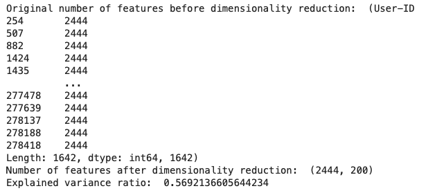
indices = book_pivot_table.index # all the user IDs

book_rating_clustering = pd.DataFrame(data=book_pivot_table_tsvd, index=indices)
print(book_rating_clustering.shape)
book_rating_clustering.head(10)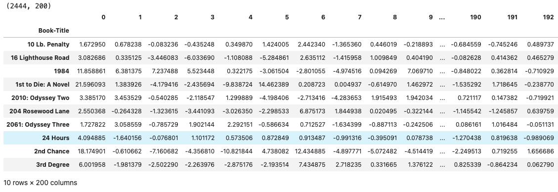
train_rate, test_rate = train_test_split(book_rating_clustering, test_size=0.2, random_state=42)
print(f'Traing set shape: {train_rate.shape}')
print('Testing set shape: {}'.format(test_rate.shape))![]()
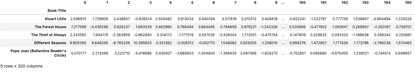
indices = test_rate.index
test_set_rating = book_pivot_table.loc[indices] # .loc[] for label-based indexing and .iloc[] for position-based indexing.
test_set_rating.head()
Exploratory Data Analysis (EDA)
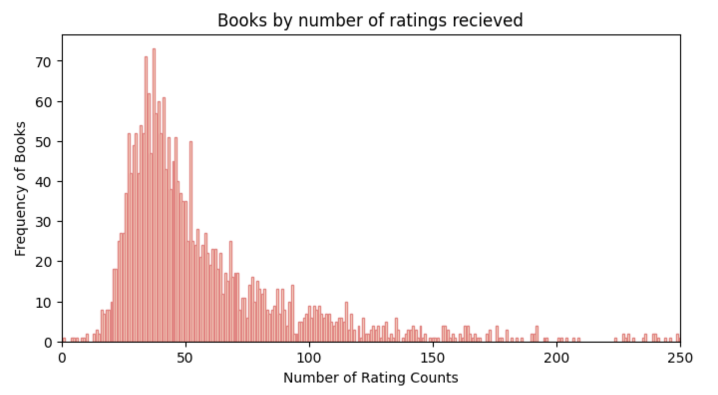
Before diving into model training, let’s explore our data further. We’ll start by examining the distribution of the number of rating counts across the books. By plotting a histogram, we can visualize how frequently different books have been rated.
# Group the data by each book and counts how many ratings each book has recieved
book_rating_counts = final_rating.groupby('Book-Title')['Book-Rating'].count()

# Calculate how many books fall into each rating count category and then sorts these counts
rating_frequencies = book_rating_counts.value_counts().sort_index()

# Plotting the histogram
plt.figure(figsize=(8, 4))
plt.bar(rating_frequencies[:500].index, rating_frequencies[:500].values, color='Cornsilk', edgecolor='LightCoral')

plt.xlim(0, 250)

# Adding titles and labels
plt.title('Books by number of ratings recieved')
plt.xlabel('Number of Rating Counts')
plt.ylabel('Frequency of Books')

# Display the plot
plt.show()
For example, below we can observe that around 25 books have received approximately 35 ratings each. The majority of books fall within the range of 25 to 75 total ratings, indicating that most books have moderate engagement from users. Interestingly, there are very few books with rating counts exceeding 150, highlighting the rarity of highly rated books in our dataset. This insight will help us better understand the characteristics of our data as we move forward.
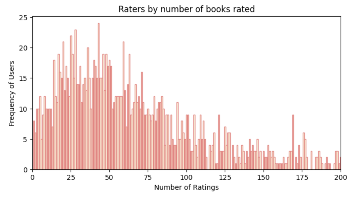
Next, let’s examine the distribution of the number of ratings provided by users. This will help us understand user engagement in our dataset.
# Group the data by each user and counts how many ratings each user has given
user_rating_counts = final_rating.groupby('User-ID')['Book-Rating'].count()

# Calculate how many users fall into each rating count category and then sorts these counts
rating_frequencies = user_rating_counts.value_counts().sort_index()


# Plotting the histogram
plt.figure(figsize=(8, 4))
plt.bar(rating_frequencies.index, rating_frequencies.values, color='Cornsilk', edgecolor='LightCoral')

plt.xlim(0, 200)

# Adding titles and labels
plt.title('Raters by number of books rated')
plt.xlabel('Number of Ratings')
plt.ylabel('Frequency of Users')

# Display the plot
plt.show()
In the plot below, we observe the frequency of users based on the number of ratings they have given. For instance, there are approximately 20 users who have voted around 37 times. Most users have given between 0 to 100 ratings, showing that casual engagement is common. Notably, the number of users who have rated more than 100 times drops sharply, with the count decreasing from about 10 to almost just 2 users. This indicates that only a small fraction of users are highly active in rating books.
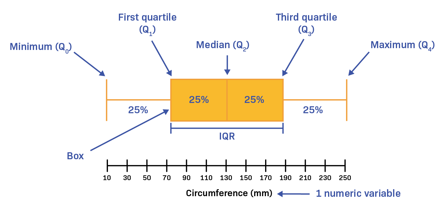
Now let’s talk about another graph: a boxplot, which is a statistical tool used to visualize the distribution of a dataset. Here are its essential components:
Box: The central part of the plot represents the interquartile range (IQR), containing the middle 50% of the data.
Median Line: A line within the box indicates the median (50th percentile) of the data.
Whiskers: Lines extending from the box to the smallest and largest values within 1.5 times the IQR from the lower and upper quartiles.
Outliers: Points outside the whiskers are considered outliers, indicating unusually high or low values.
Quartiles: The edges of the box represent the first quartile (Q1, 25th percentile) and the third quartile (Q3, 75th percentile).
A boxplot efficiently illustrates the data’s spread, central tendency, and potential outliers.
# Count the number of ratings per book
book_rating_counts = final_rating.groupby('Book-Title')['Book-Rating'].count().reset_index()

# Rename columns for clarity
book_rating_counts.columns = ['Book-Title', 'Number of Ratings']

print(book_rating_counts['Number of Ratings'].max())

# Plotting the boxplot
plt.figure(figsize=(8, 4))
sns.boxplot(x='Number of Ratings', data=book_rating_counts, color='LightCoral')
plt.xlabel('Number of Ratings per Book')
plt.title('Distribution of Number of Ratings per Book')
plt.grid(True)
plt.show()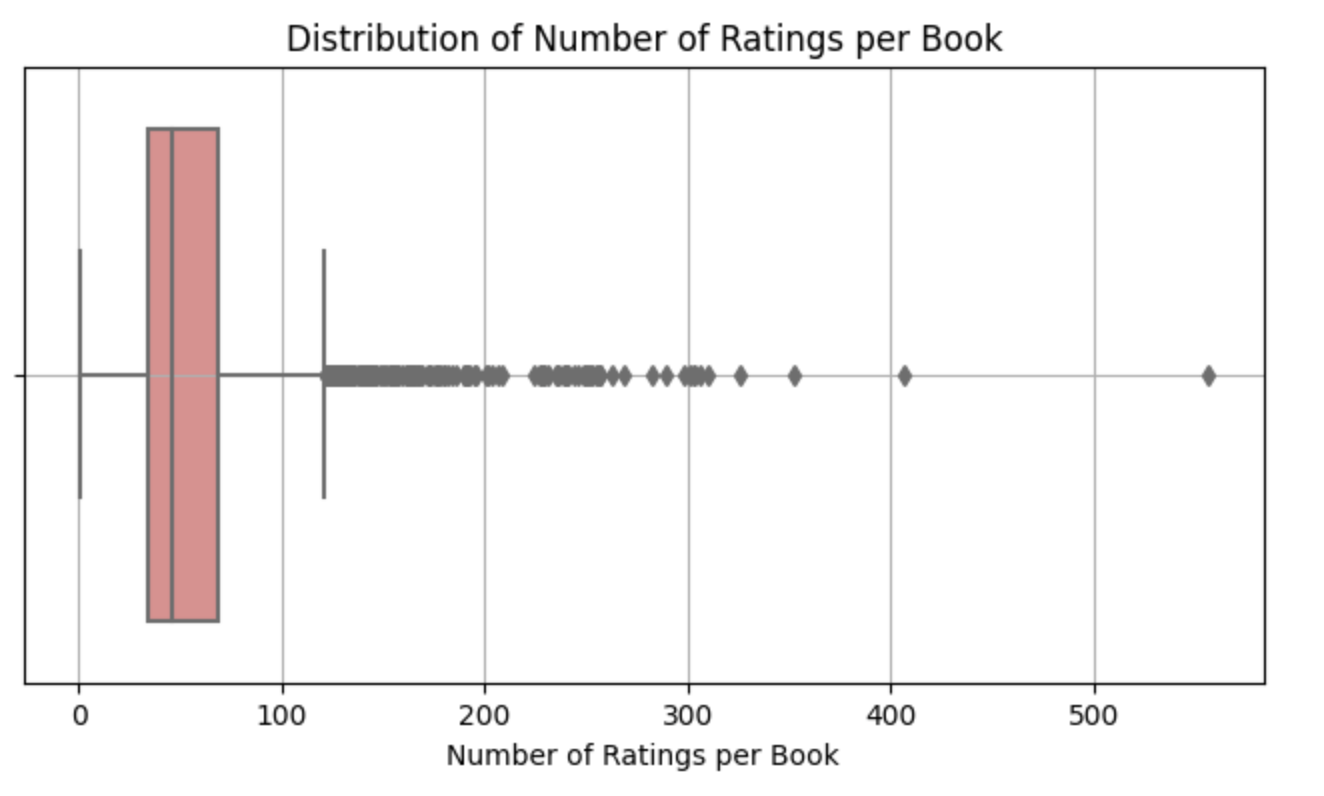
So in the plot above, we can observe that the majority of books received a bit over 100 ratings. Half of the books have at most 50 votes. Additionally, 75% of the books have up to ~75 votes. The maximum value within our fourth quartile (Q4) lies between 100 and 120, indicating that most books do not receive more than 120 votes. The minimum rating a user can give is 1, and there are outliers on the right-hand side, displayed as gray dots. These represent individual books, with one book on the far right edge having a rating as high as 556.
# Count the number of ratings per user
user_rating_counts = final_rating.groupby('User-ID')['Book-Rating'].count().reset_index()

# Rename columns for clarity
user_rating_counts.columns = ['User-ID', 'Number of Ratings']

# Plotting the boxplot
plt.figure(figsize=(8, 4))
sns.boxplot(x='Number of Ratings', data=user_rating_counts, color='LightCoral')
plt.xlabel('Number of Ratings per User')
plt.title('Distribution of Number of Ratings per User')
plt.grid(True)
plt.show()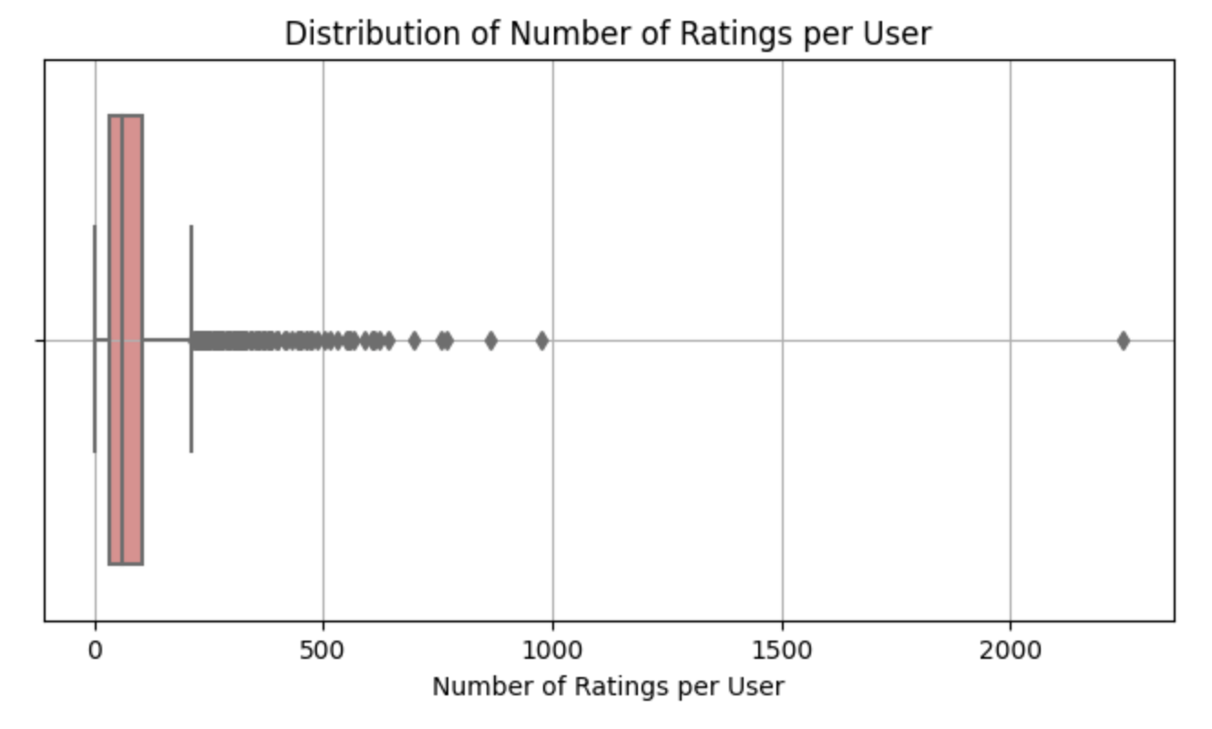
The plot for users is more condensed, with one outlier (an individual) having rated more than 2,000 books! However, the majority of voters fall within the range of 1 to just under 250 votes. Half of the voters have cast at most 60 votes, and 75% have rated at most close to 100 times. This suggests that most users don’t engage in extensive voting.
Training Machine Learning Model
Content filtering, especially when dealing with a large number of users and items, requires significant computational resources. As the number of users (U) and items (I) increases, the computational demands grow nonlinearly, primarily due to the time-intensive process of calculating similarities. The time complexity for such operations can be expressed as O(U × I), where the similarity calculations dominate the computational time.
To address these challenges, we propose using content clustering combined with neighbors’ voting. Clustering is a technique used to group similar data points into clusters. In the context of recommendation systems, clustering can help group items (e.g., books) that have similar patterns of user ratings. This reduces the computational load by allowing us to focus on clusters of similar items rather than individual item comparisons across the entire dataset.
Clustering is an unsupervised learning task, meaning we don’t have labeled data to guide the process. Instead, we aim to discover hidden patterns and relationships within the dataset. Our objective is to group books based on user rankings without any predefined categories or labels. By identifying clusters of books that have similar rating patterns, we can better understand how these books relate to each other in the eyes of users. This understanding is crucial for building an effective recommendation system that can suggest relevant items to users based on their preferences.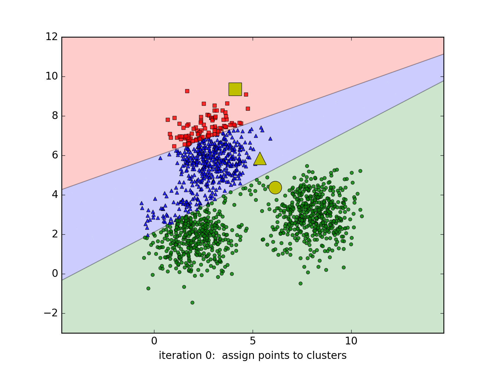
For this task, we experiment with two clustering algorithms: K-Means and Gaussian Mixture Modeling (GMM). Both are unsupervised learning techniques used for clustering, but they handle the assignment of data points to clusters differently.
K-mean Clustering
Hard Assignment: K-Means clustering operates under the assumption that each data point belongs to one and only one cluster.
Determinate Clustering: At any given point in the algorithm, we are certain about the cluster assignment of each data point. For example, if a point is assigned to the red cluster, the algorithm is fully confident in that assignment. In subsequent iterations, this assignment might change, but the certainty remains; the point will be entirely assigned to a different cluster (e.g., green). This approach is known as a “hard assignment.”
# Fit the KMeans model
clusterer_KMeans = KMeans(n_clusters=6, random_state=42).fit(train_rate)

# Transform the data to get predictions
preds_KMeans = clusterer_KMeans.predict(train_rate)

unique_labels = np.unique(preds_KMeans)
print(f"Number of clusters: {len(unique_labels)}")

KMeans_score = silhouette_score(train_rate, preds_KMeans)
print('Silhouette score for k-mean approach: ', KMeans_score)![]()
Gaussian Mixture Modeling
Soft Assignment: GMM, on the other hand, allows for uncertainty in cluster assignments. Instead of assigning a data point to a single cluster with full certainty, GMM provides probabilities for a point’s membership in multiple clusters.
Probabilistic Clustering: For instance, a data point might have a 70% probability of belonging to the red cluster, a 10% probability of being in the green cluster, and a 20% probability of being in the blue cluster. This approach is known as a “soft assignment,” where the model expresses the degree of uncertainty in cluster membership.
Iterative Refinement: GMM starts with a prior belief about the cluster assignments, and as the algorithm iterates, it continuously revises these probabilities, taking into account the uncertainty in each assignment.
# clustering books
clusterer_GM = GaussianMixture(n_components=6, random_state=42).fit(train_rate)
preds_GM = clusterer_GM.predict(train_rate)

GM_score = silhouette_score(train_rate, preds_GM)
print('Silhouette score for Gaussian Mixture approach: ', GM_score)
Silhouette scores measure how similar an object is to its own cluster compared to other clusters, providing a way to assess the quality of clustering.
In the above code snippets we used Silhouette scores to compare the performance of K-Means and Gaussian Mixture Models (GMM). The score must range from -1 to 1, with higher scores indicating better clustering—where points are more closely grouped within their own clusters and well-separated from others.
As observed, GMM (score = 0.124) outperforms K-Means (score = 0.014), as it creates more distinct and well-defined clusters.
indices = train_rate.index
preds = pd.DataFrame(data=preds_GM, columns=['cluster'], index=indices)
print(preds.shape)
for i in range(7):
  print('cluster ', i+1, ':', preds[preds['cluster'] == i+1].count())
preds.head()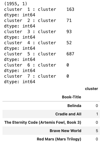
Prediction
test_preds = clusterer_GM.predict(test_rate)
test_indices = test_rate.index
test_cluster = pd.DataFrame(data=test_preds, columns=['cluster'], index=test_indices)

Test_GM_score = silhouette_score(test_rate, test_preds)

print(f'Silhouette Score for the test set is: {Test_GM_score}')
test_cluster.head()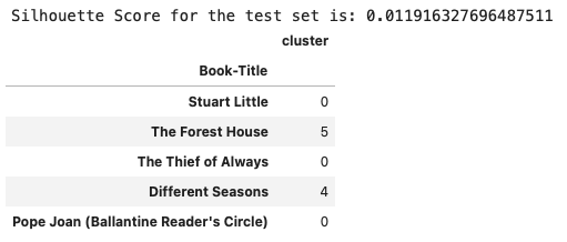
Downloading Necessary Files
Creating the App
We are using Flask, a micro web framework that we’ve previously utilized in blog 2. The project’s structure should look like this:
├── myproject
|   └── dataset
|       └── Books.csv
|       └── Ratings.csv
│   └── models
|       └── book_pivot_table.pkl
|       └── books.pkl
|       └── predicted_clusters.pkl
|   └── static/css
|       └── styles.css
|   └── templates
|       └── index.html
|       └── recommendation.html
|   └── utils.py
|   └── app.py
Software Design
We begin by collecting the name of the book that the user enjoys and wants to find similar recommendations for. Using this input, we then need our book-user table, which contains the entire dataset, as well as the predicted clusters from our clustering algorithm, and the number of recommendations the user desires.
The first step is to check if the given book exists in our dataset. Once validated, we identify the cluster to which the book belongs. With this cluster identified, we retrieve a list of all the books within that specific cluster. To find books similar in style to the one the user enjoys, we calculate the cosine similarity between the rankings of the given book and all the other books in the cluster. This similarity score helps us determine which books are closest in style and content based on user rankings. Finally, we select the top 10 books with the highest similarity scores, ensuring that the recommended books align closely with the user’s preferences. This method leverages both clustering and similarity metrics to provide personalized and relevant book recommendations.
utils.py
import numpy as np

def recommending_books(book_name, book_pivot_table, preds, n_recommendations=10):
    # Check if the book is in the pivot table
    if book_name not in book_pivot_table.index:
        return np.array([f"The book '{book_name}' is not in the dataset :/"])

    # Find the cluster of the given book
    book_cluster = preds.loc[book_name, 'cluster']

    # Get all the books in the same cluster
    cluster_books = preds[preds['cluster'] == book_cluster].index

    # Calculate similarity scores within the cluster
    book_vector = book_pivot_table.loc[book_name].values.reshape(1, -1)

    cluster_vectors = book_pivot_table.loc[cluster_books].values

    similarity_scores = np.dot(cluster_vectors, book_vector.T).flatten()

    # Sort the books by similarity scores
    similar_books_indices = np.argsort(-similarity_scores)[1:n_recommendations+1]  # Skip the first one as it's the book itself

    similar_books = cluster_books[similar_books_indices]

    return list(similar_books)
The next step is to create our Flask application file. First, we need to load our pre-trained models and data using the pickle library. Specifically, we load the pivot table of book-user interactions, the book metadata, and the predicted clusters, which are stored as pickle files.
After loading these files, we set up the initial web page using the index.html template. This page will display 12 random books with their titles and images, and also provide an interface for the user to input a book title for recommendations.
Lastly, we handle the user request by checking whether the book title exists in our pivot table. If the title exists, we call our recommending_books function to get the top 10 book recommendations. For each recommended book, we extract the title and the corresponding profile picture, then render these results through the recommendation.html template.
If the book title doesn’t exist in the dataset, an error message is displayed on the recommendation.html page.
app.py
from flask import Flask,render_template,request
import pickle
import numpy as np
from utils import recommending_books

pt = pickle.load(open('path/to/book_pivot_table.pkl','rb'))
book = pickle.load(open('path/to/books.pkl','rb'))
preds = pickle.load(open('path/to/predicted_clusters.pkl','rb'))

app = Flask(__name__)

@app.route('/')
def index():
    return render_template('index.html',
                           book_name = list(book['Book-Title'][109:121].values),
                           image = list(book['Image-URL-M'][109:121].values),
                           )

@app.route('/recommendation')
def recommendation_ui():
    return render_template('recommendation.html')

@app.route('/recommend_books', methods=['post'])
def recommendation():
    user_input = request.form.get('user_input')

    recommendations = recommending_books(user_input, pt, preds, n_recommendations=10)

    # Check if the book is not found
    if isinstance(recommendations, np.ndarray) and recommendations[0].startswith("The book"):
        return render_template('recommendation.html', error=recommendations[0])

    # Gather the data for rendering
    data = []
    for book_name in recommendations:
        item = []
        temp_df = book[book['Book-Title'] == book_name]
        item.extend(list(temp_df.drop_duplicates('Book-Title')['Book-Title'].values))
        item.extend(list(temp_df.drop_duplicates('Book-Title')['Image-URL-M'].values))
        data.append(item)
        print(item)

    return render_template('recommendation.html', data=data)


if __name__ == '__main__':
    app.run(debug=True)
Below are the templates and the static (CSS) files.
<!DOCTYPE html>
<html lang="en">
<head>
    <meta charset="UTF-8">
    <title>Book Recommendation Website</title>
    <link rel="stylesheet" href="{{ url_for('static', filename='css/styles.css') }}">
    <link rel="stylesheet" href="https://maxcdn.bootstrapcdn.com/bootstrap/4.4.1/css/bootstrap.min.css">
    <script src="https://ajax.googleapis.com/ajax/libs/jquery/3.4.1/jquery.min.js"></script>
    <script src="https://cdnjs.cloudflare.com/ajax/libs/popper.js/1.16.0/umd/popper.min.js"></script>
    <script src="https://maxcdn.bootstrapcdn.com/bootstrap/4.4.1/js/bootstrap.min.js"></script>
    <link rel="stylesheet" href="https://cdnjs.cloudflare.com/ajax/libs/font-awesome/6.0.0-beta3/css/all.min.css">
</head>
<body style="background-color:#ffe4e1">
    <nav class="navbar" style="background-color:currentColor">
        <!-- <a class="navbar-brand" style="color: white; font-size: 30px">Book Recommendation System</a> -->
        <ul class="nav navbar-nav ml-auto">
            <li><a href="/" style="color: #d8bfd8" ><i class="fas fa-home" ></i></a></li>
        </ul>
    </nav>

    <div class="container">
        <div class="row">
            <div class="col-md-12">
                <h1 class="text-blue" style="font-size: 45px; color:#4a0f6f; margin-top: 10px;margin-left:300px"><a href="/recommendation"> 💻 Type in a Book's Name... </a></h1>
            </div>

            <div class="container" style="padding-bottom: 50px;"> <!-- Add padding at the bottom -->
                <div class="row">
                    {% for i in range(book_name|length) %}
                        <div class="col-md-3" style="margin-top:50px">
                        <div class="card" style="width: 100%; height: 100%">
                            <div class="card-body" style="font-family: emoji;padding: 1.02rem">
                                <img class="card-img-top" src="{{image[i]}}" alt="Book Image"
                                style="width: 100%; height: 70%; object-fit: cover;">
                                <h4 class="text-blue" style="font-size: 20px; font-weight: bold; margin-top: 10px;">{{book_name[i]}}</h4>
                            </div>
                        </div>
                        </div>
                    {% endfor %}
                </div>
            </div>

        </div>
    </div>
</body>
</html>
<!DOCTYPE html>
<!DOCTYPE html>
<html lang="en">
<head>
<meta charset="UTF-8">
<title>Recommendation Site</title>
<link rel="stylesheet" href="{{ url_for('static', filename='css/styles.css') }}">
<link rel="stylesheet" href="https://maxcdn.bootstrapcdn.com/bootstrap/4.4.1/css/bootstrap.min.css">
<script src="https://ajax.googleapis.com/ajax/libs/jquery/3.4.1/jquery.min.js"></script>
<script src="https://cdnjs.cloudflare.com/ajax/libs/popper.js/1.16.0/umd/popper.min.js"></script>
<script src="https://maxcdn.bootstrapcdn.com/bootstrap/4.4.1/js/bootstrap.min.js"></script>
<link rel="stylesheet" href="https://cdnjs.cloudflare.com/ajax/libs/font-awesome/6.0.0-beta3/css/all.min.css">
</head>
<body style="background-color:#ffe4e1" >
<nav class="navbar" style="background-color:currentColor">
<!-- <a class="navbar-brand" style="color: white; font-size: 30px">Book Recommendation System</a> -->
<ul class="nav navbar-nav ml-auto">
<li><a href="/" style="color: #d8bfd8"><i class="fas fa-home"></i></a></li>
</ul>
</nav>
<div class="container">
<div class="row">
<div class="col-md-12">
<h4 class="text-blue" style="font-size: 35px; color:#4a0f6f; margin-top: 15px;">Recommended Books</h4>
<form action="/recommend_books" method="post" style="margin-top: 20px;">
<input name="user_input" type="text" class="form-control" placeholder="Enter a book title">
<br>
<input type="submit" class="btn btn-lg btn-warning" style="background-color: #b0e0e6; color: #4a0f6f" value="Get Recommendations">
</form>
</div>
</div>
<div class="container" style="padding-bottom: 50px;"> <!-- Add padding at the bottom -->
<div class="row">
{% if data %}
<p class="text-blue" style="font-size: 25px; margin-top: 15px;">Based on your preference, we think you might like the following books! :)</p>
<div class="row">
{% for i in data %}
<div class="col-md-3" style="margin-top:50px">
<div class="card" style="width: 100%; height: 100%">
<img class="card-img-top" src={{i[1]}} alt="Book Image">
<div class="card-body">
<h4 class="text-blue" style="font-size: 20px; font-weight: bold; margin-top: 10px;">{{i[0]}}</h4>
</div>
</div>
</div>
{% endfor %}
</div>
{% endif %}
</div>
</div>
</div>
</div>
</body>
</html>.card {
transition: transform 0.3s ease, box-shadow 0.3s ease;
}
.card:hover {
transform: scale(1.05); /* Scales up the card */
box-shadow: 0px 4px 20px rgba(0, 0, 0, 0.2); /* Adds a shadow effect */
}
.card-body {
padding: 1.02rem;
font-family: emoji;
}
.card-img-top {
width: 100%;
height: 70%;
object-fit: cover;
}
.text-blue {
color: #4a0f6f; /* Example color */
}Virtual Environment Setup and Run
After completing the programming part, it’s time to execute! Follow the steps below in your preferred terminal (make sure you are in your project directory first):
Create a virtual environment:
mamba create -n env_name -c conda-forgeActivate the environment:
mamba activate env_nameFind the Python path:
which pythonSet the Python interpreter:
On Mac press
command + shift + pOn Windows press
Ctrl + Shift + PThen select “Python: Select Interpreter” and paste the Python path you found in the previous step
Install required packages, including Flask:
mamba install flaskRun the app:
python app.py
Results and Limitations
Here’s a short demo of our simple, functional app currently under development. You can, of course, add more features and functionalities as needed.
In this project, we endeavored to implement content-based filtering, a form of recommendation system, on a book dataset. The core objective was to utilize unsupervised algorithms like K-Means and the Gaussian Mixture Model to cluster book titles based on their relevance or irrelevance to each other. This allows us to suggest books that are similar to the one a user selects for a recommendation.
This “closeness” between books is considered a latent factor—an underlying variable that is not directly observable but inferred from other measurable variables, such as rankings. Latent factors are commonly used in recommendation systems and matrix factorization techniques like Singular Value Decomposition (SVD), which we employed in our approach.
While we successfully achieved our goal, our approach has limitations. Specifically, our system can only recognize and recommend books that already exist in our dataset. In other words, if the book title provided by the user does not exist in our clusters, we cannot generate a recommendation. This limitation is particularly evident when a new user joins the system or a new book is added to the archive, as there is no existing information—no rankings, no history—about these new entries. This is a known issue in recommendation systems, often referred to as the “Cold Start” problem, where content filtering struggles with new books, and collaborative filtering cannot produce recommendations for new users. Addressing this challenge could be a fruitful area for further exploration, with many academic papers available to guide the way.
That concludes this project. I hope it was worth your time and that you learned something new along the way, just as I did while working on it. As always, feel free to share your feedback or any comments you might have.
Until the next blog, happy coding!
Links to my code: