How to Build a Music Genre Classifier Using Hugging Face Transformers and Gradio

In this blog, we will build a music genre classification system using the GTZAN dataset to identify the genre of a given audio track.

Have you ever been curious about how machine learning models classify music genres? What features in the dataset are useful for the model’s understanding? And how can you deploy your trained model for users? If these questions have crossed your mind, then keep reading as I guide you through everything you need to quickly deploy a music classification app. By the end of this post, you will have a fully functional music genre classification model capable of predicting the genre of any audio track. You will also have a Gradio-based interactive interface to test and visualize the model’s predictions, and the model will be ready for deployment using the Hugging Face Hub.

Load and Prepare the Dataset

We start by loading the GTZAN dataset using the datasets library and split it into training and test sets. The reason for using GTZAN is that it’s a popular dataset containing 1,000 songs for music genre classification. Each song is a 30-second clip from one of 10 genres of music, spanning blues to rock.

from datasets import load_dataset

# Load the GTZAN dataset
gtzan = load_dataset('marsyas/gtzan', 'all')

# Split the dataset into training and test sets
gtzan = gtzan['train'].train_test_split(seed=42, shuffle=True, test_size=0.1)

# How does the dataset look like
print(gtzan)

# Create a function to convert genre ID to genre name
id2label_fn = gtzan['train'].features['genre'].int2str

# Example of converting a genre ID to genre name
print(id2label_fn(gtzan['train']['genre'][1]))

Output

DatasetDict({
    train: Dataset({
        features: ['file', 'audio', 'genre'],
        num_rows: 899
    })
    test: Dataset({
        features: ['file', 'audio', 'genre'],
        num_rows: 100
    })
})
classical

Explanation

• Loading Dataset: load_dataset('marsyas/gtzan', 'all') loads the GTZAN dataset.
• Splitting Dataset: train_test_split splits the dataset into training and validation sets with 90% training and 10% validation.
• Label Conversion Function: int2str() maps numeric genre IDs to their corresponding genre names (human-readable names).

Generate Audio Samples with Gradio

As you have seen in the previous section, our dataset contains three types of features: file, audio, and genre. We learned about genre and now let’s have a closer look at audio and figure out what’s inside of it.

gtzan["train"][0]["audio"]

Output

{'path': '/root/.cache/huggingface/datasets/downloads/extracted/5022b0984afa7334ff9a3c60566280b08b5179d4ac96a628052bada7d8940244/genres/pop/pop.00098.wav',
 'array': array([ 0.10720825,  
                  0.16122437,  
                  0.28585815, 
                  ..., 
                  -0.22924805,
                  -0.20629883, 
                  -0.11334229]
                ),
 'sampling_rate': 22050}

As you can see, the audio file is represented as 1-dimensional NumPy array. But what does the value of array represent? And what is sampling_rate?

Sampling and Sampling Rate

In signal processing, sampling refers to the process of converting a continuous signal (such as sound) into a discrete signal by taking periodic samples.

Wikipedia article: Sampling (signal_processing)

In our example of audio sampling, sampling rate (or sampling frequency) refers to the number of samples of audio carried per second. It is usually measured in Hertz (Hz). To put it in perspective, standard media consumption has a sampling rate of 44,100 Hz, meaning it takes 44,100 samples per second. In comparison, high-resolution audio has a sampling rate of 192,000 Hz (192 kHz). For training speech models, a commonly used sampling rate is 16,000 Hz (16 kHz).

Amplitude

When we talk about the sampling rate in digital audio, we refer to how often samples are taken. But what do these samples actually represent?

Sound is produced by variations in air pressure at frequencies that are audible to humans. The amplitude of a sound measures the sound pressure level at any given moment and is expressed in decibels (dB). Amplitude is perceived as loudness; for example, a normal speaking voice is typically under 60 dB, while a rock concert can reach around 125 dB, which is near the upper limit of human hearing.

In digital audio, each sample captures the amplitude of the audio wave at a specific point in time. For instance, in our sample data gtzan["train"][0]["audio"], each value in the array represents the amplitude at a particular timestep. For these songs, the sampling rate is 22,050 Hz, which means there are 22,050 amplitude values recorded per second.

One thing to remember is that all audio examples in your dataset have the same sampling rate for any audio-related task. If you intend to use custom audio data to fine-tune a pre-trained model, the sampling rate of your data should match the sampling rate of the data used to pre-train the model. The sampling rate determines the time interval between successive audio samples, therefore impacting the temporal resolution of the audio data.

To read more on this topic click here.

Gradio

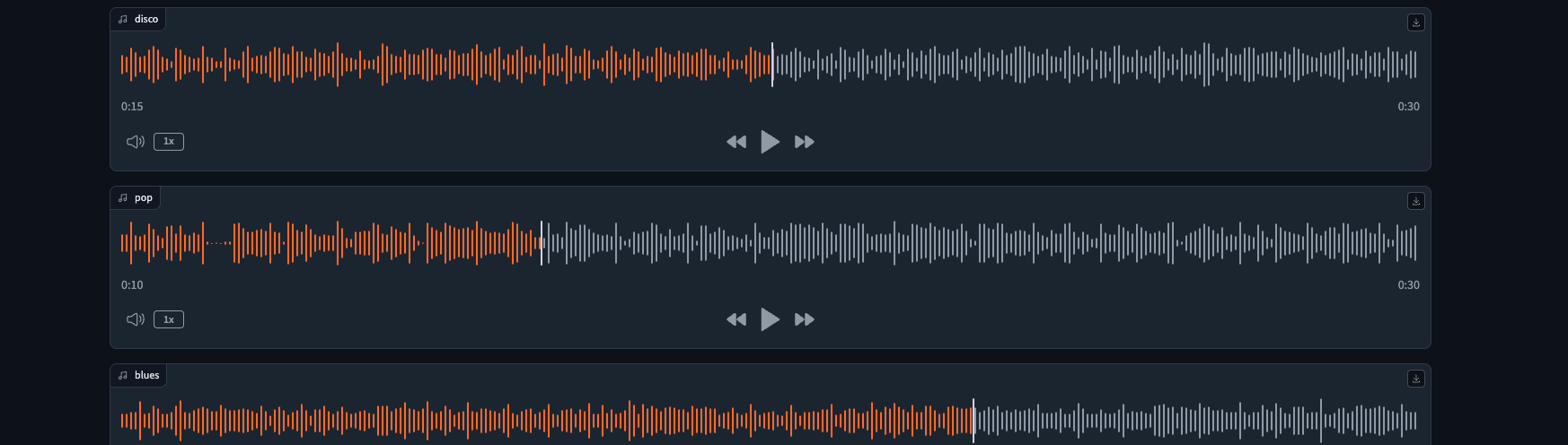
Now that we better understand our dataset let’s create a aimple and interactive UI with the Blocks API to visualize some audio samples and their labels.

import gradio as gr

# Function to generate an audio sample
def generate_audio():
    example = gtzan["train"].shuffle()[0]
    audio = example["audio"]
    return (audio["sampling_rate"], audio["array"]), id2label_fn(example["genre"])

# Create a Gradio interface to display audio samples
with gr.Blocks() as demo:
    with gr.Column():
        for _ in range(4):
            audio, label = generate_audio()
            output = gr.Audio(audio, label=label)

# Launch the Gradio demo
demo.launch(debug=True)

Output

Explanation

• Generating Audio: generate_audio() randomly selects and returns an audio sample from the training set.
• Gradio Interface: Gradio Blocks and Column create a layout to display audio samples. gr.Audio adds audio players with labels to the interface.
• Launching Interface: demo.launch(debug=True) starts the Gradio interface for interaction.

Feature Extraction

Just as tokenization is essential in NLP, audio and speech models need input encoded in a processable format. In 🤗 Transformers, this is handled by the model’s feature extractor. The AutoFeatureExtractor class automatically selects the right feature extractor for a given model. Let’s see how to process our audio files by instantiating the feature extractor for DistilHuBERT from the pre-trained checkpoint:

from transformers import AutoFeatureExtractor

# Load a pre-trained feature extractor
model_id = 'ntu-spml/distilhubert'
feature_extractor = AutoFeatureExtractor.from_pretrained(
    model_id,
    do_normalize=True,
    return_attention_mask=True
)

# Get the sampling rate from the feature extractor
sampling_rate = feature_extractor.sampling_rate
sampling_rate

Output

16000

Explanation

• Loading Feature Extractor: AutoFeatureExtractor.from_pretrained loads a pre-trained feature extractor model.
• Sampling Rate: feature_extractor.sampling_rate retrieves the sampling rate needed for the audio data.

Preprocess the Dataset

We preprocess the audio data to match the input requirements of the model by converting audio samples to the desired format and sampling rate.

from datasets import Audio

# Cast the audio column to match the feature extractor's sampling rate
gtzan = gtzan.cast_column('audio', Audio(sampling_rate=sampling_rate))

gtzan["train"][0]

Below we can verify that the sampling rate is downsampled to 16 kHz. 🤗 Datasets will resample the audio file in real-time as each audio sample is loaded:

Output

{
    "file": "~/.cache/huggingface/datasets/downloads/extracted/fa06ce46130d3467683100aca945d6deafb642315765a784456e1d81c94715a8/genres/pop/pop.00098.wav",
    "audio": {
        "path": "~/.cache/huggingface/datasets/downloads/extracted/fa06ce46130d3467683100aca945d6deafb642315765a784456e1d81c94715a8/genres/pop/pop.00098.wav",
        "array": array(
            [
                0.0873509,
                0.20183384,
                0.4790867,
                ...,
                -0.18743178,
                -0.23294401,
                -0.13517427,
            ],
            dtype=float32,
        ),
        "sampling_rate": 16000,
    },
    "genre": 7,
}

What we have just done is that we’ve provided the sampling rate of our audio data to our feature extractor. This is a crucial step as the feature extractor verifies whether the sampling rate of our audio data matches the model’s expected rate. If there were a mismatch, we would need to up-sample or down-sample the audio data to align with the model’s required sampling rate.

After processing our resampled audio files, the final step is to create a function that can be applied to all examples in the dataset. Since we want the audio clips to be 30 seconds long, we will truncate any longer clips using the max_length and truncation arguments of the feature extractor.

# Function to preprocess the audio data
max_duration = 30.0

def preprocess_function(examples):
    audio_arrays = [x["array"] for x in examples["audio"]]
    inputs = feature_extractor(
        audio_arrays,
        sampling_rate=feature_extractor.sampling_rate,
        max_length=int(feature_extractor.sampling_rate * max_duration),
        truncation=True,
        return_attention_mask=True,
    )
    return inputs

# Apply the preprocessing function to the dataset
gtzan_encoded = gtzan.map(
    preprocess_function,
    remove_columns=["audio", "file"],
    batched=True,
    batch_size=100, # by default is 1000
    num_proc=1,
)
gtzan_encoded

Output

DatasetDict({
    train: Dataset({
        features: ['genre', 'input_values', 'attention_mask'],
        num_rows: 899
    })
    test: Dataset({
        features: ['genre', 'input_values', 'attention_mask'],
        num_rows: 100
    })
})

Explanation

• Preprocessing Function: preprocess_function truncates or pads audio samples to a fixed length, normalizes them, and creates attention masks.
• Applying Function: gtzan.map applies the preprocessing function to the entire dataset.

feature_extractor provides a dictionary containing two arrays: input_values and attention_mask. That is why we see them as new columns for our features.

sample = gtzan["train"][0]["audio"]

inputs = feature_extractor(sample["array"], sampling_rate=sample["sampling_rate"])

print(f"inputs keys: {list(inputs.keys())}")

inputs keys: ['input_values', 'attention_mask']

For a simpler training process, we’ve excluded the audio and file columns from the dataset. Instead, the dataset now includes an input_values column with encoded audio files, an attention_mask column with binary masks (0 or 1) indicating padded areas in the audio input, and a genre column with corresponding labels or targets.

Prepare Labels

We need to rename the genre column to label to enable the Trainer to process the class labels.

gtzan_encoded = gtzan_encoded.rename_column("genre", "label")

# Create mappings from IDs to labels and vice versa
id2label = {str(i): id2label_fn(i) for i in range(len(gtzan_encoded["train"].features["label"].names))}
label2id = {v: k for k, v in id2label.items()}

id2label

Output

{ '0': 'blues',
  '1': 'classical',
  '2': 'country',
  '3': 'disco',
  '4': 'hiphop',
  '5': 'jazz',
  '6': 'metal',
  '7': 'pop',
  '8': 'reggae',
  '9': 'rock'
}

Explanation

• Renaming Column: rename_column("genre", "label") renames the genre column to label.
• Creating Mappings: id2label and label2id create dictionaries to map genre IDs to names and vice versa.

Load and Fine-tune the Model

We load a pre-trained audio classification model and fine-tune it on the GTZAN dataset.

from transformers import AutoModelForAudioClassification

# Load a pre-trained audio classification model
num_labels = len(id2label)

model = AutoModelForAudioClassification.from_pretrained(
    model_id,
    num_labels=num_labels,
    label2id=label2id,
    id2label=id2label,
)

The next step is optional but advised. We basically link our notebook to the 🤗 Hub. The main advantage of doing so is to ensure that no model checkpoint is lost during the training process. You can get your Hub authentication token (permission: write) from here :

# Login to Hugging Face Hub (optional)
from huggingface_hub import notebook_login

notebook_login()

Output

Next step, we define the training arguments (e.g. batch size, number of epochs, learning rate, etc.)

# Define training arguments
from transformers import TrainingArguments

model_name = model_id.split("/")[-1]
batch_size = 8
gradient_accumulation_steps = 1
num_train_epochs = 10

training_args = TrainingArguments(
    f"{model_name}-finetuned-gtzan",
    evaluation_strategy="epoch",
    save_strategy="epoch",
    learning_rate=5e-5,
    per_device_train_batch_size=batch_size,
    gradient_accumulation_steps=gradient_accumulation_steps,
    per_device_eval_batch_size=batch_size,
    num_train_epochs=num_train_epochs,
    warmup_ratio=0.1,
    logging_steps=5,
    load_best_model_at_end=True,
    metric_for_best_model="accuracy",
    fp16=True,
    push_to_hub=True,
)

Explanation

• Loading Model: AutoModelForAudioClassification.from_pretrained loads a pre-trained model for audio classification.
• Training Arguments: TrainingArguments defines parameters for training, such as batch size, learning rate, number of epochs, and strategies for evaluation and saving.

Training and Evaluation

Lastly, we define a function to compute metrics and create a trainer to handle the training process.

import evaluate
import numpy as np

# Load the accuracy metric
metric = evaluate.load("accuracy")

# Function to compute accuracy
def compute_metrics(eval_pred):
    predictions = np.argmax(eval_pred.predictions, axis=1)
    return metric.compute(predictions=predictions, references=eval_pred.label_ids)

# Initialize the trainer
from transformers import Trainer

trainer = Trainer(
    model,
    training_args,
    train_dataset=gtzan_encoded["train"],
    eval_dataset=gtzan_encoded["test"],
    tokenizer=feature_extractor,
    compute_metrics=compute_metrics,
)

# Train the model
trainer.train()

Output

| Epoch | Training Loss | Validation Loss | Accuracy |
|:-----:|:-------------:|:---------------:|:--------:|
| 1.0   |   1.950200    |    1.817256     | 0.51     |
| 2.0   |   1.158000    |    1.208284     | 0.66     |
| 3.0   |   1.044900    |    0.998169     | 0.72     |
| 4.0   |   0.655100    |    0.852473     | 0.74     |
| 5.0   |   0.611300    |    0.669133     | 0.79     |
| 6.0   |   0.383300    |    0.565036     | 0.86     |
| 7.0   |   0.329900    |    0.623365     | 0.80     |
| 8.0   |   0.114100    |    0.555879     | 0.81     |
| 9.0   |   0.135600    |    0.572448     | 0.80     |
| 10.0  |   0.105100    |    0.580898     | 0.79     |

Using the free tier GPU on Google Colab, we successfully trained our model in about 1 hour. With just 10 epochs and 899 training examples, we achieved an evaluation accuracy of up to 86%. To further optimize model performance, we could increase the number of epochs or apply regularization techniques such as dropout.

Inference

Now that we have our trained model, we can automatically submit our checkpoint to the leaderboard. You can modify the following values to fit your dataset, language, and model name:

kwargs = {
    "dataset_tags": "marsyas/gtzan",
    "dataset": "GTZAN",
    "model_name": f"{model_name}-finetuned-gtzan",
    "finetuned_from": model_id,
    "tasks": "audio-classification",
}

The training results can now be uploaded to the Hub through the .push_to_hub command:

trainer.push_to_hub(**kwargs)

By following these steps, you built a complete system for music genre classification using the GTZAN dataset, Gradio for interactive visualization, and Hugging Face Transformers for model training and inference.

Gradio Demo

Now that we built our music classification model trained on GTZAN dataset, we can showcase it on Gradio. We first need to load up fine-tuned checkpoint using the pipeline() class:

from transformers import pipeline

model_id = "toobarah/distilhubert-finetuned-gtzan"
pipe = pipeline("audio-classification", model=model_id)

Next, we defined a function that processes an audio file through the pipeline. The pipeline handles loading the file, resampling it to the correct rate, and running inference with the model. The model’s predictions are then formatted as a dictionary for display.

def classify_audio(filepath):
    preds = pipe(filepath)
    outputs = {}
    for p in preds:
        outputs[p["label"]] = p["score"]
    return outputs

Final step, we launch the Gradio demo by calling the function we just created:

import gradio as gr

demo = gr.Interface(
    fn=classify_audio, inputs=gr.Audio(type="filepath"), outputs=gr.Label()
)
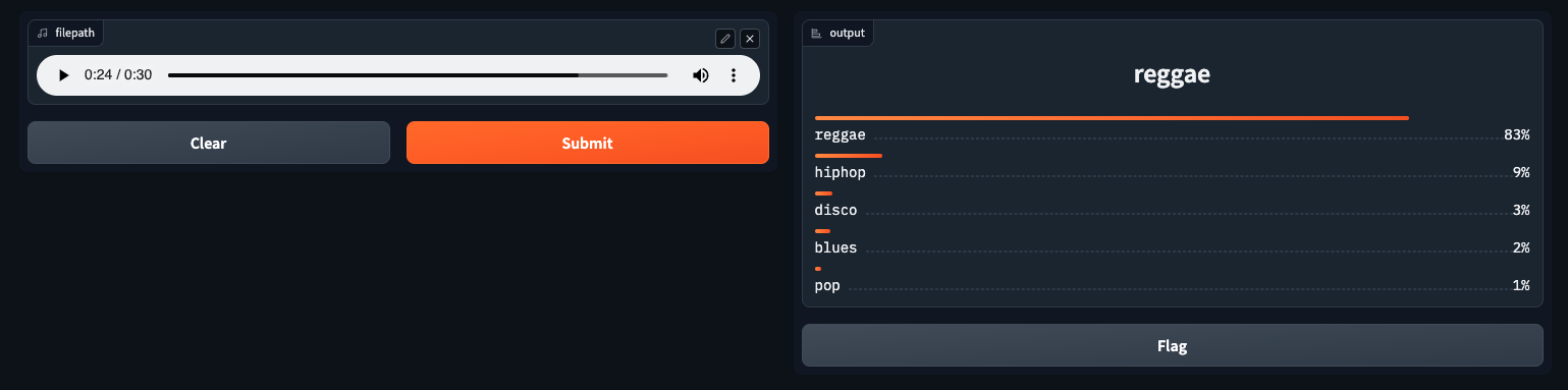
demo.launch(debug=True)

* If you get an ImportError after running the last cell, try downgrading your Gradio using the following command:

pip install gradio==3.47.1

Otherwise, you should see a window pop up as shown below! Go ahead, upload some music, test your model, and enjoy!

Conclusion

This tutorial was a step-by-step guide for fine-tuning the DistilHuBERT model for a music classification task. It has also been a learning journey for me, and I drew much inspiration from the work of the Hugging Face audio course as I began this project. I hope I was able to explain the steps clearly and that they were easy for you to follow. Every step shown here can be applied to any audio classification task, so if you’re interested in exploring other datasets or models, I recommend checking out other examples in the 🤗 Transformers repository.

For access to all the code shared here in one file, click on this Colab file. Happy coding! :)